← back

Mixture-of-Experts

Mixture-of-expert (MoE) is rapidly becoming one of the core components of big, performant LLMs. DeepSeek-V3 uses it, Alibaba's Qwen-3 has an MoE version, and the latest Llama 4 Maverick is a mixture-of-experts model.

In short, a mixture-of-experts is a way to scale model capacity without proportionally increasing compute cost during inference. Instead of activating all model parameters for every input, an MoE architecture contains multiple “experts”, where only a small subset (e.g., 2 out of 64) is activated for each token. This sparse activation allows the model to have many more parameters overall while keeping the per-token compute roughly constant.

This blog post provides an overview of different popular mixtures of experts, starting from their infancy to the latest DeepSeek MoEs.

Mixture-of-Experts in the 90s

In 1991, Jacobs, Jordan, Nowlan and Hinton published the paper "Adaptive Mixtures of Local Experts". In the paper, they presented a new idea: a supervised learning process composed of many separate networks - each of which learns to handle a subset of the complete training dataset. They demonstrate that this process can work on a 'vowel discrimination' task, which works by separating the core task into appropriate subtasks, each of which can be solved by an expert network. The key idea is described as follows:

If we know in advance that a set of training cases may be naturally divided into subsets that correspond to distinct subtasks, interference can be reduced by using a system composed of several different "expert" networks plus a gating network that decides which of the experts should be used for each training case.

The gating mechanism allocates a new case to one or a few experts, and, if the output is incorrect, the weight changes are localized to these experts (and the gating network). This makes each expert subnetwork specialised - experts are 'local' as their weights are decoupled from the weights of other experts. The gating network outputs a softmax weight vector, and the final prediction is the weighted sum of all expert outputs. As such, there is no hard selection of a limited number of experts.

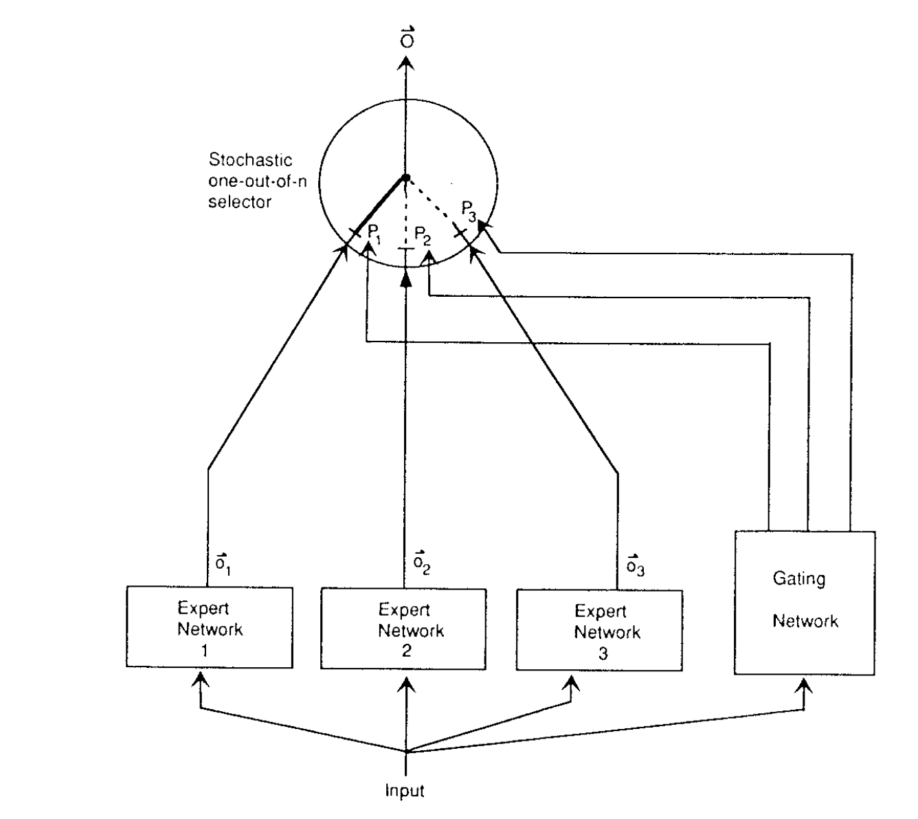
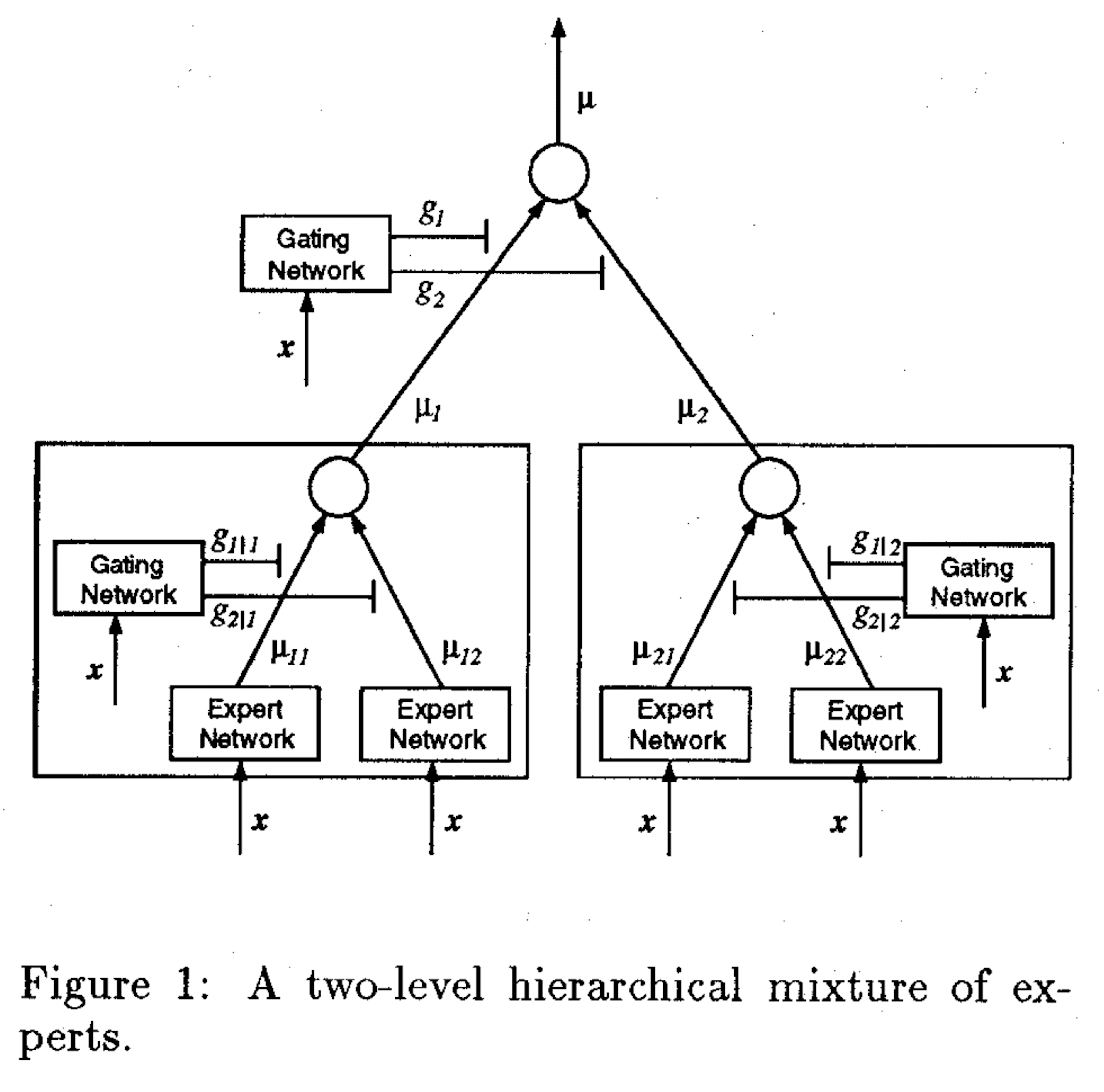
Diagram overview of the '91 paper (left) and the '93 paper (right)

In 1993, Jordan and Jacobs published "Hierarchical mixtures of experts and the EM algorithm", in which they make the structure of the mixture of experts hierarchical - if the network is a tree, the gating network sits at the root. Because they present their network as a tree, each subtree can have a gating network with more subnetworks as well. Comparatively, in the 1991 paper, the routing part of the network is a separate function at the same level as the experts (see image). These two papers form the basis of the mixture of experts architecture: a network with a gating mechanism that determines which part of the network to active based on the input, and then a subnetwork with $N$ experts.

Remarkable how ideas like this from more than 30 years ago shape today's models.

Scaling to 137B parameters in 2017

So let's step forward in time — what remains of the original idea? A lot! However, pretty much all MoEs from now on have a few things in common:

1. How can we scale MoEs to models with billions or even trillions of parameters? MoEs allow you to scale to models with an insane number of parameters, but only if some of the model's capacity is not used all the time. We'll see that this is usually fixed by top-k gating—only activating a select number of experts.
2. How do we avoid expert collapse, that is, the risk that the model converges to using only a few experts during training? If we naively train MoEs with top-k gating, the winning expert gets the only non-zero gradient for that token. Its parameters (and the router weight that points to it) move in a direction that further increases that probability.

In addition, many MoE papers will be authored by Noam Shazeer :).

In his seminal 2017 paper Outrageously Large Neural Networks: The Sparsely-Gated Mixture-of-Experts Layer, the two questions above are answered with:

1. Top-k gating, which means that only the top $k$ experts with the highest softmax probability are used. As a result, a lot of computation is saved — we only need to activate the top $k$ (e.g., top-2) out of thousand experts. The benefit of this is that the batch size can be increased significantly compared to when the full model would be used.
2. Noisy gating: they add tunable gaussian noise to the gating network. This helps to avoid expert collapse as there will be more dispersion in the softmax output.

Moreover, they use a 'soft constraint' in the loss function, taken from Bengio et al. (2015) (Emmanuel Bengio, not Yoshua or Samy). You will see this more often — a constraint on the loss to encourage effective expert routing. More precisely, in this paper, for each batch, they define the importance of an expert to be the batchwise sum of the gate values for that expert, something like this:

# Shape: (batch_size, num_experts)
G = [
  [0.7, 0.2, 0.1, 0.0],  # input 1
  [0.6, 0.3, 0.1, 0.0],  # input 2
  [0.1, 0.1, 0.8, 0.0],  # input 3
  ...
]
W_importance = torch.sum(G, dim=0)
# Result: [X0, X1, X2, X3] ← how much each expert was used in total

These values are then used in an additional loss term $L_{importance}$, which takes the square of the coefficient of variation of the set of importance values, multiplied by a hand-tuned scaling factor $w_{importance}$. This additional loss encourages all experts to have equal importance.

$$L_{\text {importance }}(X)=w_{\text {importance }} \cdot C V(\text { Importance }(X))^2$$

Where CV is

$$\begin{equation} \mathrm{CV}(v)=\frac{\text { StandardDeviation }(v)}{\operatorname{Mean}(v)} \end{equation}$$

As such, a perfectly balanced setup (standard deviation = 0) would lead to a low loss value, whereas a high standard deviation will lead to a higher $L_{importance}$ value (see the widget below, generated by ChatGPT).

In addition to $L_{importance}$, a second loss term $L_{load}$ is also added to encourage an equal load of samples (see Appendix A of the paper).

Taken together, this approach laid the groundwork for massively scalable sparse MoE models that power today's largest language models, such as GShard, GLaM, Switch Transformer, and the MoE variants used by DeepSeek.

MoEs in 2020-2022: GShard, GLaM

GShard

After the Shazeer paper and several scaling law papers, the deep learning community increasingly focused on scaling models. Whereas the 2017 MoE paper trained a model with 137B parameters, GShard: Scaling Giant Models with Conditional Computation and Automatic Sharding (2020, Google, Shazeer as co-author) presented models with 600B parameters. While most of the paper focuses on efficiently implementing parallel training at scale, the MoE described differs as it is one of the first scaled transformer MoE models. More precisely, every other feed-forward layer in the transformer is replaced with an MoE with fixed top-2 gating. The output of the MoE layer is the weighted average of all outputs from all selected experts. To train this efficiently at scale, GShard proposes a new concept called expert capacity, which enforces that the number of tokens processed by one expert is below some uniform threshold (while processing many tokens in parallel). By keeping a running counter of how many tokens are dispatched to an expert, we track when a expert has exceeded its capacity. When this is the case, the token is considered an overflowed token and is set to be the zero vector, and its representation is passed on to the next layer via residual connections.

As the auxiliary loss, Gshard uses the following setup:

$\ell_{\mathrm{aux}}=\frac{1}{E} \sum_{e=1}^E \underbrace{\frac{c_e}{S}}_{\substack{\text { actual } \\ \text { load }}} \cdot \underbrace{m_e}_{\substack{\text { soft } \\ \text { load }}}$

Where $c_e / S$ defines the fraction of tokens $S$ routed to expert $e$, and $m_e$ the probability distribution of the gating mechanism. We use both as $c_e / S$ is not differentiable.

GLaM: Efficient Scaling of Language Models with Mixture-of-Experts (2021) further scales this setup to a model with 1.2T parameters. Mixtral of Experts, Mistral's MoE, which got some popularity in 2024, mentions GShard as the main inspiration for their MoE implementation. They use an MoE in every layer instead of every other layer, but Mistral does not provide more details on how they further train or implement the MoE.

Post ChatGPT MoEs

Switch Transformer (2022)

Google keeps iterating on the MoE architecture, and in 2022 they publish Switch Transformers: Scaling to Trillion Parameter Models with Simple and Efficient Sparsity. GShard and GLaM assumed that top-2 gating was required as a trade-off between predictive performance and the training/serving efficiency of the model. The idea was that using more experts would lead to better model performance but at the cost of computing cost. However, Switch Transformers breaks with this idea and uses top-1 instead of top-k routing. This has three benefits:

1. Computation is reduced as we only route to a single expert.
2. As a result, the batch size can be halved.
3. The routing implementation is simplified and communication costs are reduced.

Like GShard, they use the expert capacity mechanism to balance the distribution of tokens across experts. The result is a model that achieves higher performance than a standard MoE transformer given the same compute budget.

ST-Moe (2022)

As we've seen so far: auxiliary losses are helpful in encouraging expert balancing. However, they can also lead to training instabilities. For example, logits in the gating mechanism can become very large, leading to training instabilities.

Stable Transferable MoE (ST-MoE), published in ST-MoE: Designing Stable and Transferable Sparse Expert Models introduces a router z-loss to fix this. The loss is defined as follows:

$L_z(x)=\frac{1}{B} \sum_{i=1}^B\left(\log \sum_{j=1}^N e^{x_j^{(i)}}\right)^2$

where $B$ is the number of tokens, $N$ is the number of experts, and $x \in \mathcal{R}^{B \times N}$ are the logits going into the router. The loss penalises large logits; it can be seen as a more smooth, integrated and differentiable version of logit clipping.

DeepSeek MoEs

We've now seen that training MoEs requires a careful combination of different loss functions and expert capacity setups. However, we are still using simple top-1 or top-2 gating. This can be seen as suboptimal; assigning a token to just a single expert means, high-level, that the token will be used in one particular way. What if we could route one token to more than two experts? This should allow each expert to decompose and learn knowledge in different ways.

This is the core idea of DeepSeekMoE: Towards Ultimate Expert Specialization in Mixture-of-Experts Language Models (2024). Specifically:

• each expert FFN is segmented into $m$ smaller experts by reducing the FFN intermediate dimension to $\frac{1}{m}$ times its original size
• Now that each expert is smaller, we can multiply the number of activated experts by $m$, keeping the same computational cost.

The above leads to many more combinations of activated experts - with 16 experts, top-2 routing has $\binom{16}{2} = 120$ combinations. By splitting each expert into 4 smaller experts, there are now $\binom{64}{8}=4,426,165,368$ potential combinations.

In addition to more experts, DeepSeek MoE adds shared experts that are always activated. The motivation behind this change is that different experts generally need some common knowledge or information. If we do not always activate a few select experts, each expert would have to learn this knowledge, leading to a redundancy in expert capacity. To maintain a constant computational cost, the number of activated experts among the other routed experts is decreased by the number of shared experts.

DeepSeek is famous for efficiency optimisations, and this MoE paper is no exception. The standard expert-balancing loss keeps per-expert utilisation flat when there is exactly one expert per GPU. DeepSeekMoE breaks that one-to-one mapping by packing many small experts onto each GPU. That optimisation exposes a new failure mode: an apparently balanced set of experts can still result in a lopsided device utilisation. To fix this, they introduce a second, higher-level regulariser:

$\mathcal{L}_{\text {DevBal }}=\alpha_2 \sum_{i=1}^D f_i^{\prime} P_i^{\prime}, \quad f_i^{\prime}=\frac{1}{\left|\mathcal{E}_i\right|} \sum_{j \in \mathcal{E}_i} f_j, \quad P_i^{\prime}=\sum_{j \in \mathcal{E}_i} P_j$

• $D$: number of devices.
• $\mathcal{E}_i$ : set of experts on device $i$.
• $f_i^{\prime}$ : mean routed-token fraction for device $i$.
• $P_i^{\prime}$ : total routing probability mass assigned to that device.

Empirically, DeepSeek sets the scaling factor for this loss higher than the one for the standard expert balancing (0.05 vs. 0.003). In other words, they pay more to equalise GPUs than to equalise individual experts.

By scaling the above setup, we can obtain performance evaluations for different model scales:

• The setup described above leads to a comparable performance with GShard 2.9B, which has 1.5x expert parameters and computation.
• A scaled 16B model achieves comparable performance with LLaMA2 7B, with only 40% of computations.
• A model scaled even more to 145B parameters is comparable with DeepSeek 67B, while only using 28.5% of computations.

DeepSeek-V3 MoE: Auxiliary-Loss-Free Load Balancing

The above setup sounds like an improvement upon the previously obtained results. But DeepSeek keeps DeepSeeking — in August 2024, they published Auxiliary-Loss-Free Load Balancing Strategy for Mixture-of-Experts which describes a technique later used in DeepSeek-V3. The main problem the authors try to adjust is the downside of using many losses, as they introduce gradients that conflict with the language modelling objective, decreasing model performance. In the plot below, $MaxVio$ is the maximal violation, a metric to quantify the degree of load balance of an MoE layer:

$MaxVio=\frac{\max _i \operatorname{Load}_i-\overline{\operatorname{Load}_i}}{\overline{\operatorname{Load}_i}}$

where $\text { Load }_i$ represents the number of tokens assigned to the $i$-th expert, and $\overline{\text { Load }_i}$ denotes the expected expert load under perfect load balance.

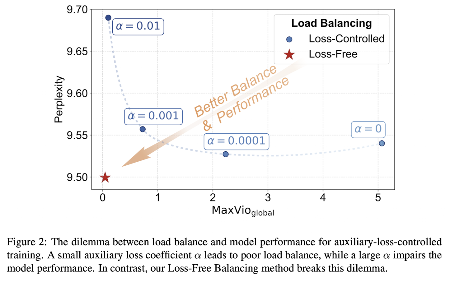
We can see that better load balancing, achieved using a higher expert balance loss coefficient, results in worse model performance (higher perplexity), whereas worse load balancing results in a better model.

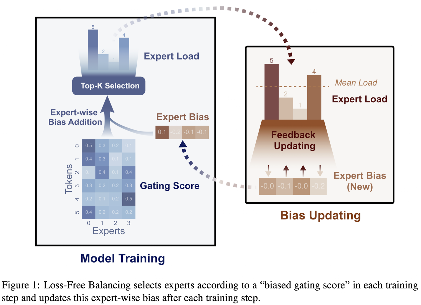
Auxiliary loss-free training breaks this dilemma, by creating a balancing strategy not affecting the gradients. How is this done? Before the top-K routing decision, Loss-Free Balancing applies biases per expert to the original routing scores, producing biased gating scores. At every training step, we update the biases based on the expert load of previous training tokens; biases of frequently used experts will be small, whereas the biases of rarely used experts will be increased. These biased gating scores will then be used to determine how to route tokens. The biases are not actually used when the outputs are combined based on the weights of the gating mechanism; they are just used to select more diverse experts.

The bias $b$ for expert $i$ is computed as follows:

1. Count the number of assigned tokens $c_i$ for each expert, and the average number $\overline{c_i}$;
2. Calculate the load violation error $e_i=\overline{c_i}-c_i$;
3. Update $\mathbf{b}_i$ by $b_i=b_i+u * \operatorname{sign}\left(e_i\right)$

$u$ is a hyperparameter set to 0.001.

The above algorithm is surprisingly simple, yet is proven to be effective. No more complicated loss functions!

Model Size	Load-Balancing Method	Validation Perplexity	MaxVioglobal
1 B	Loss-Controlled	9.56	0.72
	Loss-Free	9.50	0.04
3 B	Loss-Controlled	7.97	0.52
	Loss-Free	7.92	0.04

Summary

MoE training is more complicated than simply splitting your model into several experts and adding a gating mechanism. Top-K gating makes stable training more difficult as we have to overcome routing collapse. Various techniques have been proposed to fix routing collapse, most commonly with auxiliary loss functions and an expert capacity mechanism. Auxiliary Loss-Free Load Balancing, used in DeepSeek-V3, breaks this pattern by using simple biased gating scores.

If you liked this blog post, feel free to share it or follow me on LinkedIn or Twitter.